Police Shootings USA 2015-2021
Marta Kowalczyk
1. Introduction
This project aims to analyze police shootings in the United States between 2015 and 2021. Police use of lethal force has been a significant topic of public discourse and policy debate, particularly concerning its disproportionate impact on specific demographic groups.
By examining data over a six-year period, this analysis seeks to uncover trends, patterns, and potential disparities in the occurrence of police shootings.
Research questions:
- How do race, gender, and age influence the likelihood of being involved in a fatal police shooting?
- Are certain demographic groups more likely to be armed during police shootings?
- Does race or age influence the likelihood of fleeing?
- How have police shootings trends changed over time from 2015 to 2021? Do any particular years or months show spikes in incidents?
- What is the relationship between being armed or showing signs of mental illness and the manner of death in police shootings?
- Are there geographic hotspots (by states) where police shootings occur more frequently? How does this correlate with other factors?
The exploratory data analysis (EDA) and statistical tests will be performed using Python, while data visualization will be carried out in Power BI for clear and insightful presentation.
2. Data Description
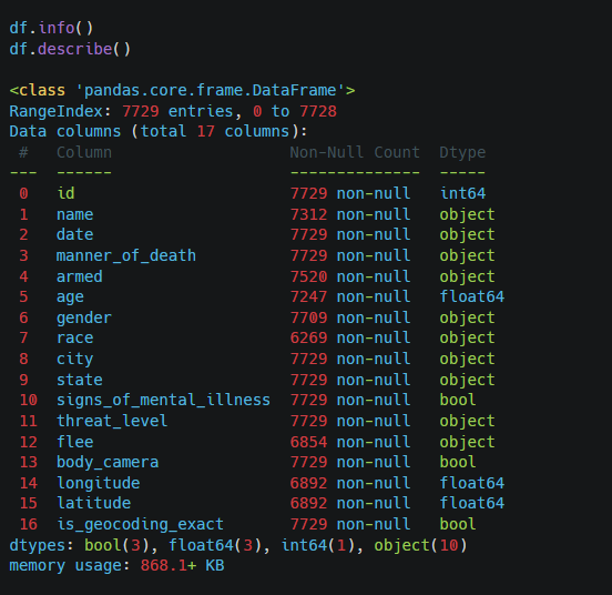
This dataset was found on Kaggle page (https://www.kaggle.com/datasets/ramjasmaurya/us-police-shootings-from-20152022/data). It was chosen as it offers the lists of people killed by law enforcement in the United States. The dataset utilized for this analysis contains 7,729 rows and 17 columns. Each row corresponds to an individual data entry, while the columns represent different attributes or variables captured in the dataset.
- id: Serial No.
- name: Name of the victim that got shot or tasered by Police.
- date: Date of the occurance.
- manner_of_death: The manner of death. Categorical variable.
- armed: If the victim was armed or not. Categorical variable.
- age: Age of the victim.
- gender: Gender of the victim. Categorical variable.
- race: Ethnicity of victim. Categorical variable.
- city: City.
- state: State. Categorical variable.
- signs_of_mental_illness: If victim showed signs of mental illness. Categorical variable.
- threat_level: Level of threat on Police. Categorical variable.
- flee: If the victim tried to flee. Categorical variable.
- body_camera: If the Police has a body camera. Categorical variable.
- longitude: Longitude of location.
- latitude: Latitude of location.
- is_geocoding_exact: Location available exact or not. Categorical variable.
3. Data Preprocessing
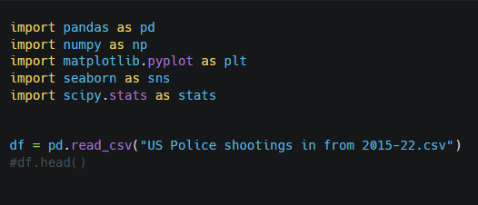
Import of Libraries and Dataset
Preliminary Data Exploration
| Id | Age | Longitude | Latitude | |
|---|---|---|---|---|
| count | 7729 | 7247 | 6892 | 6892 |
| mean | 3865 | 37.178971 | -97.059875 | 36.682999 |
| std | 2231.314448 | 12.966191 | 16.595557 | 5.402749 |
| min | 1 | 2 | -160.007 | 19.498 |
| 25% | 1933 | 27 | -112.039 | 33.48 |
| 50% | 3865 | 35 | -94.226 | 36.1045 |
| 75% | 5797 | 45 | -83.07325 | 40.03225 |
| max | 7729 | 92 | -67.867 | 71.301 |
Comment:
There are 7729 rows in this dataset.
The descriptive statistics of age variable suggest that the younger victim was 2 and the older one – 92 years old. The mean (37) and the median (35) are close to each other, indicating that the age distribution is approximately normal (Gaussian).
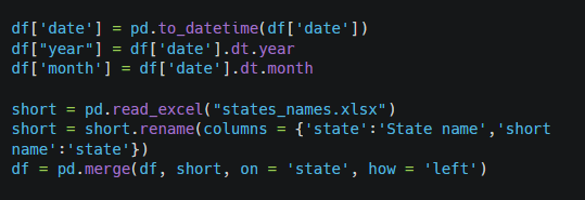
Extraction of the month and a year from the date. Merging other table to get the full name of the State.
Handling Missing Values
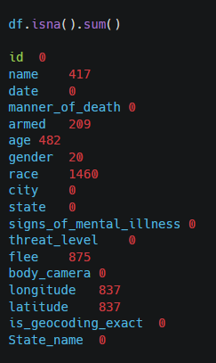
Comment: There are many missing values in the important variables for this analysis such as the age, race or flee.
Due to this fact, I decided to drop missing values instead of trying to replace them with medians or means, which could impact the data and lead to wrong conclusions. I will create copies of df to analyse the variables separately, as I want to preserve as much of the data as possible.
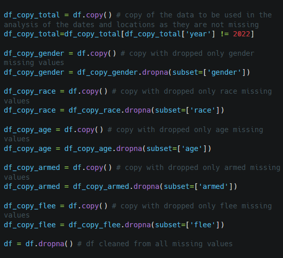
Comment: After dropping the missing values, there are 4986 observations left in df. I will use copies to analyze the variables separately to not lose the meaningfull information.
Dropping the column „id” and the observations from 2022 (not full year in this dataset – I will analyze only full years 2015-2021).
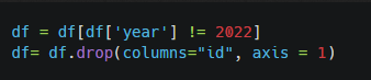
Comment: Column «No» with indexing dropped.
Check of Duplicated Rows
Comment: The result is 0 – there are no duplicated observations.
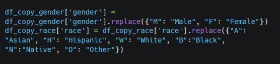
Replacing the Categorical Values
4. Exploratory Data Analysis – EDA
4.1 How do race, gender, and age influence the likelihood of being involved in a fatal police shooting?
Age
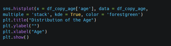
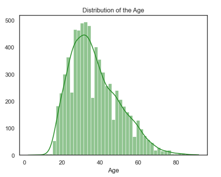
Comment: Most of the individuals are between 25 and 40 years old. This histogram is left-skewed – there are many outliers of old age.
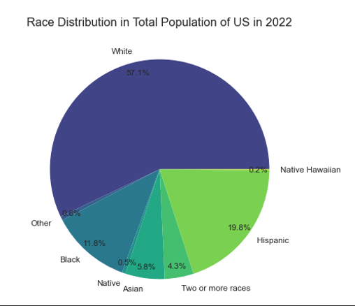
Race
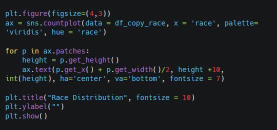
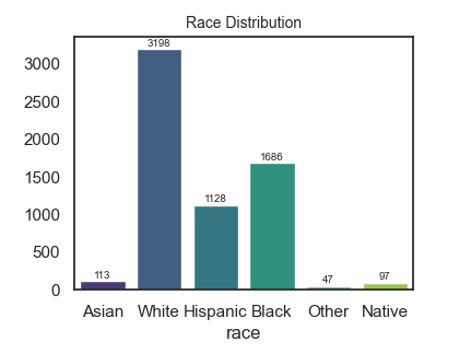
Comment: The distribution of race in the dataset closely reflects the demographic composition of the general U.S. population:
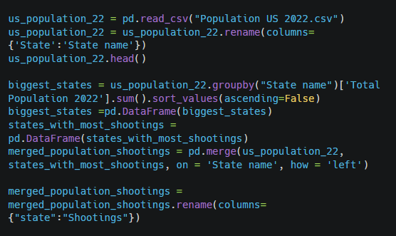
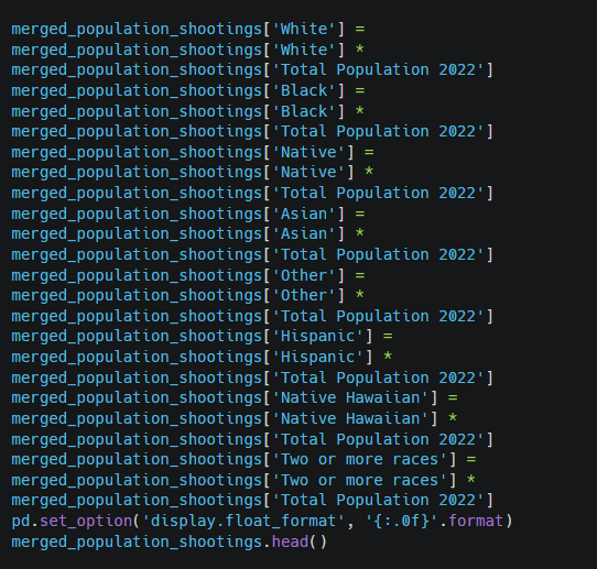
I am going to compare the numbers of shootings per race with the total population of US (report copied from Wikipedia (https://en.wikipedia.org/wiki/Demographics_of_the_United_States), contain the data from 2022).
First, I am converting the % into numbers:
| State Name | Total Population 2022 | White | Black | Native | Asian | Naitve Hawaiian | Other | Two or more Races | Hispanic | Shootings |
|---|---|---|---|---|---|---|---|---|---|---|
| Alabama | 5074296 | 3252624 | 1299020 | 15223 | 76114 | 0 | 20297 | 167452 | 248641 | 130 |
| Alaska | 733583 | 421077 | 20540 | 93165 | 44749 | 14672 | 3668 | 78493 | 56486 | 49 |
| Arizona | 7359197 | 3812064 | 323805 | 242854 | 257572 | 14718 | 36796 | 287009 | 2391739 | 313 |
| Arkansas | 3045637 | 2055805 | 435526 | 12183 | 48730 | 15228 | 12183 | 213195 | 255834 | 97 |
| California | 39029344 | 13152889 | 2029526 | 117088 | 5971490 | 117088 | 234176 | 1678262 | 15728826 | 1028 |
Now, I am going to create barchart of total population to compare with brchart of shootings:

Below the results to compare:
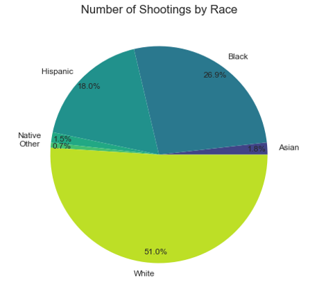
| Race | % of Total Population | % of Shootings | Radio |
|---|---|---|---|
| Asian | 5,80% | 1,80% | 31,03% |
| Black | 11,80% | 26,90% | 227,97% |
| Hispanic | 19,80% | 18,00% | 90,91% |
| Native | 0,50% | 1,55% | 310,00% |
| Other | 5,10% | 0,75% | 14,71% |
| White | 57,10% | 51,00% | 89,32% |
The analysis of the ratios between the percentage of police shootings and the percentage of the U.S. population for each racial group reveals significant disparities.
*Black individuals are highly overrepresented, with a ratio of 227%, indicating that they are involved in police shootings more than twice as often as expected based on their share of the population.
*Native Americans also show a significant overrepresentation, with a ratio of 310%, suggesting they face an even higher likelihood of being involved in police shootings relative to their population size.
*Asian individuals, with a ratio of 31%, and Other racial groups, with 14.7%, are notably underrepresented in police shootings, suggesting they are far less likely to be involved compared to their population share.
*Hispanic individuals have a ratio of 90.91%, which is relatively close to parity, meaning their representation in police shootings is slightly less than expected based on population.
*White individuals, with a ratio of 89.31%, are also underrepresented in police shootings relative to their population size, though not as significantly as other groups.
These findings highlight stark racial disparities, particularly for Black and Native American communities, indicating that certain racial groups are disproportionately impacted by police shootings in the U.S.
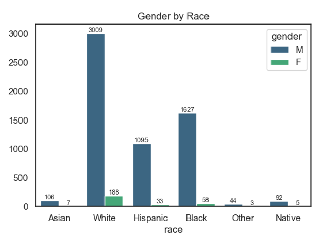
Gender
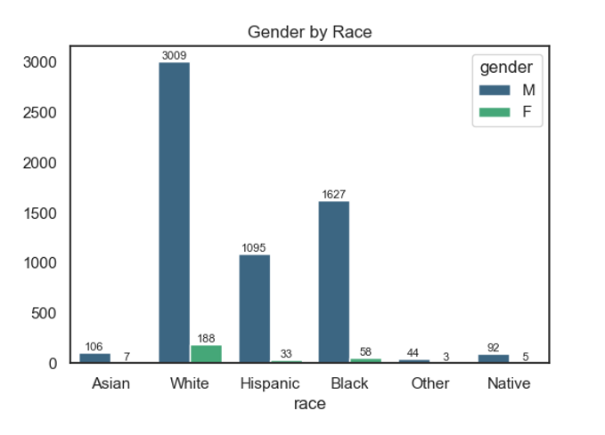
Comment: The chart shows that in police shootings, males overwhelmingly dominate across all racial groups, especially among White (3009 males vs. 188 females) and Black victims (1627 males vs. 58 females). Other racial groups, like Hispanic, Asian, Other, and Native, also follow this trend, with males being much more frequently involved than females. This indicates a strong gender disparity in victims of police shootings, with males being far more affected across all races.
Race vs Gender
Comment:
The chart shows that in police shootings, males overwhelmingly dominate across all racial groups, especially among White (3009 males vs. 188 females) and Black victims (1627 males vs. 58 females). Other racial groups, like Hispanic, Asian, Other, and Native, also follow this trend, with males being much more frequently involved than females. This indicates a strong gender disparity in victims of police shootings, with males being far more affected across all races.
Race vs Age
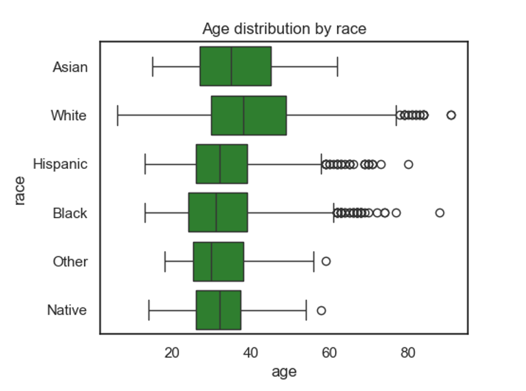
Comment:
The boxplot shows the distribution of age among victims of police shootings, categorized by race. Most racial groups have victims primarily aged 20 to 50, with notable outliers in the older age ranges, particularly among White and Hispanic groups. The Native group has the youngest distribution, while the White group has the broadest age range with numerous older outliers.
Race vs Gender
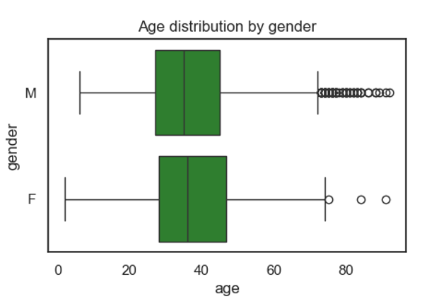
Comment:
The age distributions for both genders are quite similar, with the central tendency around 30 to 45 years old. The presence of outliers in both plots indicates that there are some individuals with ages significantly different from the majority.
Gender and Age of Victims
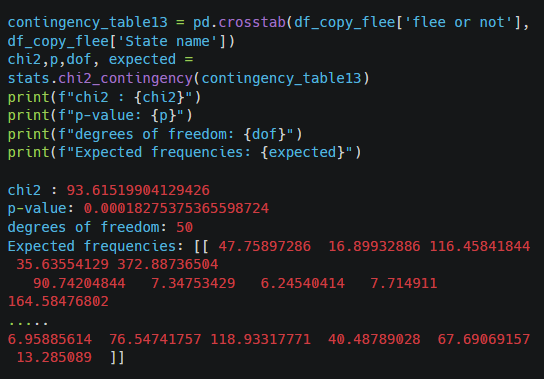
Chi-squared Test
Null Hypothesis: There is no association between age and gender.
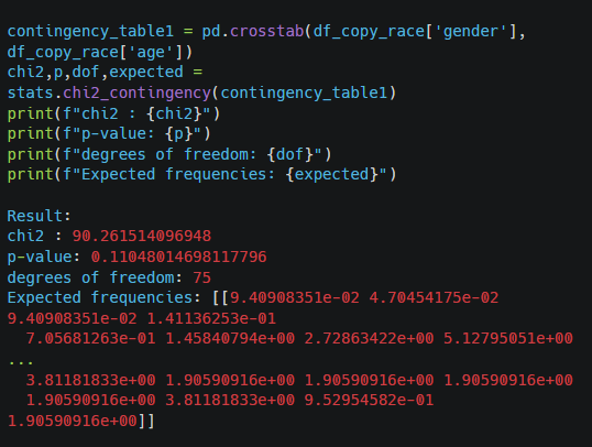
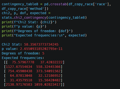
Comment: Since the p-value is less than 0.05, we reject the null hypothesis. This means that there is a statistically significant association between race and gender among the victims of police shootings in this dataset. Gender and race are not independent.
Race and Age of Victims
Chi-squared Test
Null Hypothesis: There is no association between race and age.
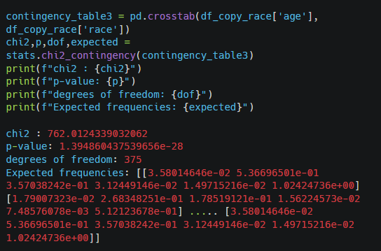
Comment: With a p-value of 1.39, which is greater than the typical significance level (e.g., 0.05), we fail to reject the null hypothesis. This suggests that there is no statistically significant association between race and age of the victims in this dataset.
– How do race, gender, and age influence the likelihood of being involved in a fatal police shooting?
The analysis of the ratios between the percentage of police shootings and the percentage of the U.S. population for each racial group reveals significant disparities – black individuals and native americans are involved in police shootings more than expected in relation to their population size.
Males are disproportionately represented in fatal police shootings compared to females. Males overwhelmingly dominate across all racial groups, especially among White (3009 males vs. 188 females) and Black victims (1627 males vs. 58 females).
Most racial groups have victims primarily aged 20 to 50, with notable outliers in the older age ranges.
The Native group has the youngest distribution, while the White group has the broadest age range with numerous older outliers. The age distributions for both genders are quite similar, with the central tendency around 30 to 45 years old. The Chi-square tests suggests that there is a statistically significant association between race and gender among the victims.
4.2 Are certain demographic groups more likely to be armed during police shootings?
Armed
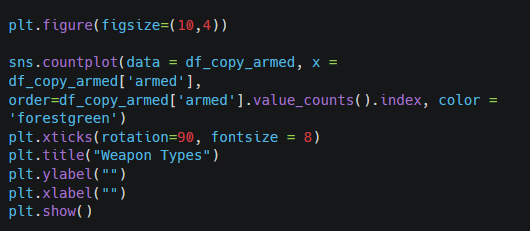
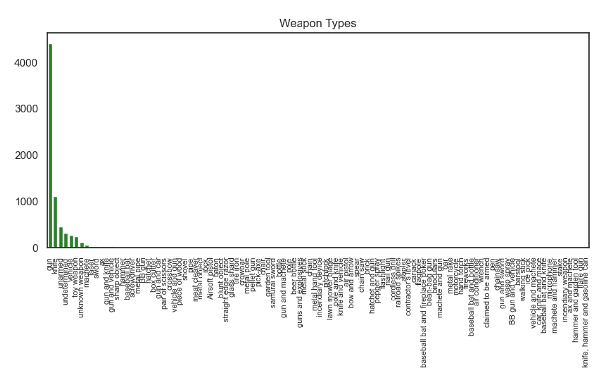
Comment:
The majority of victims in this dataset was armed with a gun. Other popular weapons seem to be knife, toy weapon, vehicle and unnamed items.
Armed vs Age
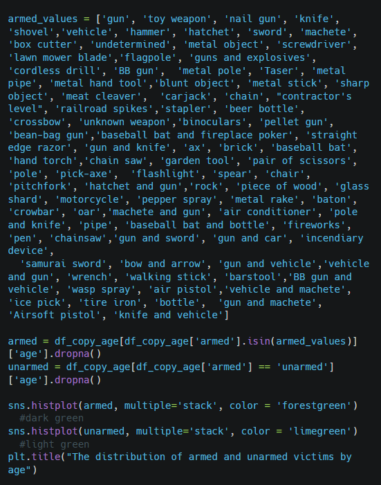
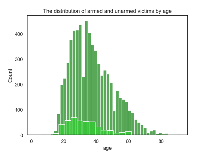
Comment:
· The majority of victims, whether armed or unarmed, are relatively young, concentrated in the 20-40 year range.
· Armed victims outnumber unarmed victims across all age groups, especially in the younger age ranges.
· After 40 years of age, the number of both armed and unarmed victims decreases significantly, but the trend is more pronounced for unarmed victims
Gender vs Armed
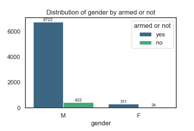
Comment:
The data shows a significant gender disparity, with males being overwhelmingly more involved in police shootings than females. There were 6,722 armed and 433 unarmed males, compared to 311 armed and 34 unarmed females.
This suggests that males are not only more likely to be involved in police shootings but also more likely to be armed at the time of the incident. The proportion of unarmed individuals among males is greater compared to females, but both genders have a much higher representation among armed individuals.
Race vs Armed
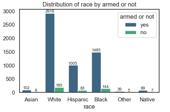
Comment:
As detected in univariate analysis, White and Black individuals have the highest representation in police shootings. Although White individuals account for the highest number of armed cases, Black individuals show a higher ratio of unarmed cases compared to other groups. Hispanic individuals also have a noticeable presence in police shootings, with armed cases being significantly higher than unarmed cases.
Armed vs Age
Chi-squared Test
Null Hypothesis: There is no association between age and being armed.
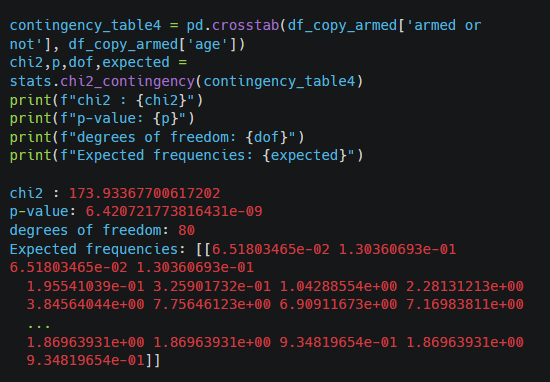
Comment: A p-value this small (6.42e-09 (which is 0.00000000642)) strongly suggests that we should reject the null hypothesis. This means there is evidence to conclude that age is associated with the likelihood of being armed in the data.
Armed vs Gender
Chi-squared Test
Null Hypothesis: There is no association between gender and being armed.
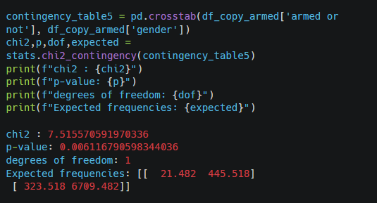
Comment: The p-value (0.0061) indicates a significant association between gender and being armed.
Therefore, gender does play a role in whether an individual is likely to be armed in this dataset. This result might suggest that men are more likely to be armed compared to women, as implied by the observed frequencies being significantly different from the expected ones
Armed vs Race
Chi-squared Test
Null Hypothesis: There is no association between race and being armed.
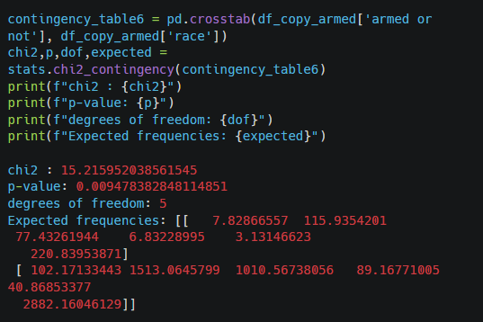
Comment:
A p-value this small (0.009) strongly suggests that we should reject the null hypothesis. This means there is evidence to conclude that race is associated with the likelihood of being armed in the data.
– Are certain demographic groups more likely to be armed during police shootings?
The Chi-square test showed that there is association between being armed and a race in this dataset. White individuals account for the highest number of armed cases, Black individuals show a higher ratio of unarmed cases.
Also gender and age seem to be strongly associated with being armed. Males are not only more likely to be involved in police shootings but also more likely to be armed at the time of the incident. Armed victims outnumber unarmed victims across all age groups, especially in the younger age ranges (20-40 years).
4.3 Does race or age influence the likelihood of fleeing?
Flee
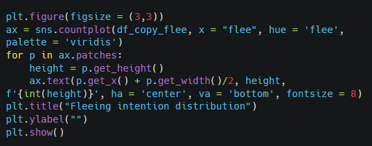
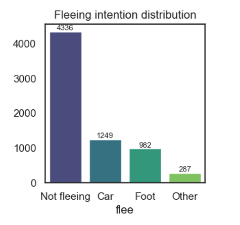
Comment: The chart illustrates the various manners in which victims attempted to flee from the police. The majority of individuals did not attempt to flee. Among those who did, 1,249 fled by vehicle, 962 on foot, and the remaining 287 employed other methods of escape.
Age vs Flee
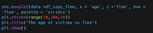
Comment: The median age of victims who did not flee is relatively higher compared to the other categories, approximately around 40-45 years old. The median age for victims fleeing by car is around 35-40 years old. The median age for victims fleeing on foot is lower, around 30-35 years. Victims using other fleeing methods have a median age similar to those fleeing by foot, around 30-35 years.
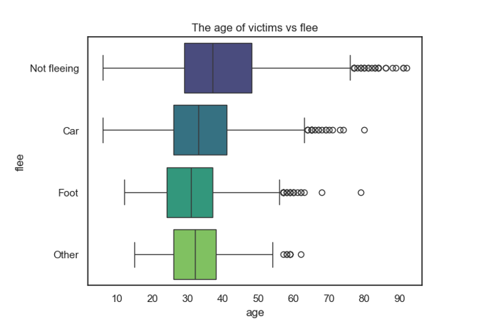
Race vs Flee
Comment: The data highlights that Black individuals had the highest percentage of fleeing attempts (39%), while Asian individuals had the lowest (21%). Most other racial groups fell within the 29%–36% range, with Whites having a lower proportion compared to Hispanic and Black individuals. This suggests varying tendencies to flee depending on racial group, with Black individuals being more likely to attempt escape compared to other races.
Race vs Flee
Chi-squared Test
Null Hypothesis: There is no association between race and attempt to flee.
Comment:
This is a very small p-value (less than 0.05), which means we reject the null hypothesis. There is strong evidence to suggest an association between race and the likelihood of attempting to flee.
Age vs Flee
Chi-squared Test
Null Hypothesis: There is no association between race and attempt to flee.
Comment:
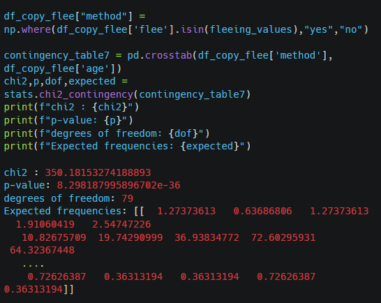
There is a significant association between age and the likelihood of attempting to flee (p < 0.05). The analysis suggests that different age groups behave differently when it comes to fleeing from the police. This association implies that age might influence whether individuals choose to flee or not.
– Does race or age influence the likelihood of fleeing?
The Chi-square tests showed that both race and age affect the intension of fleeing by the victims. Black individuals had the highest percentage of fleeing attempts (39%), while Asian individuals had the lowest (21%). Most other racial groups fell within the 29%–36% range. In case of the age, individuals who did not attempt to flee tend to be older, while those fleeing by foot or other methods tend to be younger.
4.4 How have police shootings trends changed over time from 2015 to 2021?
Do any particular years or months show spikes in incidents?
Years
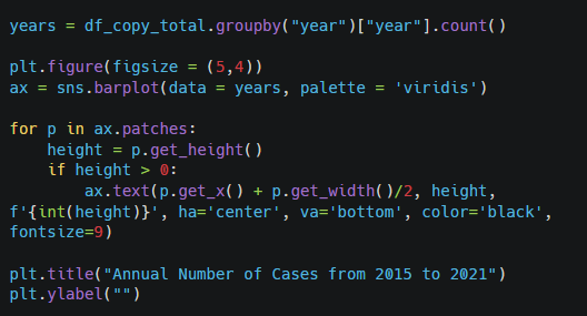
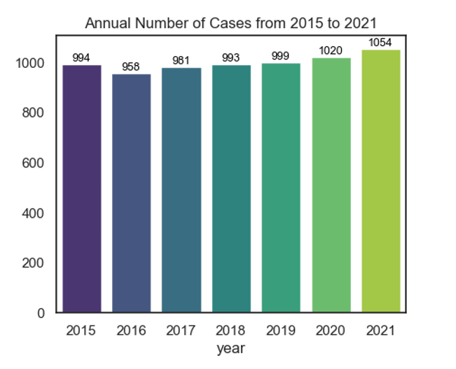
Comment: We can observe a relatively stable trend in the number of cases over the years, with slight fluctuations. The year 2016 has the lowest number of cases (958), while 2021 shows the highest number (1054).
Notably, after a small decrease in 2016, the number of cases increases slightly, peaking in 2021. The numbers appear to be consistently high, which highlights the persistent issue of police shootings in the country, without any significant reduction across the years.
Months
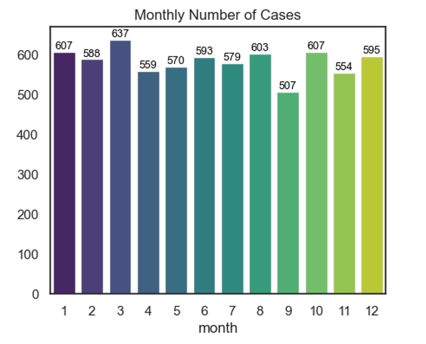
Comment:
The month of March has the highest number of cases at 637. January and November also have relatively high counts, both at 607.
The number of cases is fairly consistent, typically ranging between 550 and 600, with slight fluctuations.
The chart shows a dip in September, but after this low point, the number of cases begins to rise again, peaking in November.
There doesn’t appear to be a clear seasonal pattern, but the months of spring (March) and fall (November) seem to see higher case counts.
– How have police shootings trends changed over time from 2015 to 2021? Do any particular years or months show spikes in incidents?
The overall trend in police shootings between 2015 and 2021 remains relatively stable, with no significant reductions observed. After a slight decrease in 2016, the number of cases gradually increases, peaking in 2021. This consistency highlights the ongoing and persistent nature of the issue across the years.
On a monthly basis, March stands out with the highest number of incidents, while September consistently shows lower counts in comparison to other months. This variation suggests that certain times of the year may experience spikes in police-related incidents.
4.5 What is the relationship between being armed or showing signs of mental illness and the manner of death in police shootings?
Signs of Mental Illness
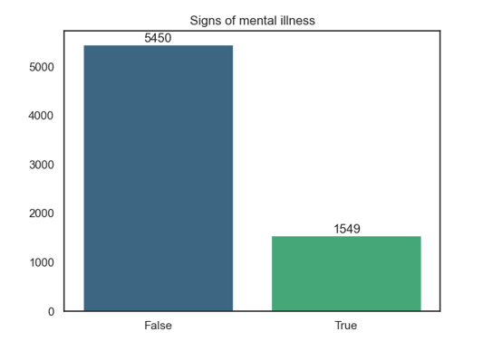
Comment:
The chart highlights that in the majority of police shootings, the victims did not display signs of mental illness, with those exhibiting mental illness making up a smaller but notable portion of the total incidents. This could suggest that mental illness plays a role in a subset of police encounters but is not a predominant factor across all incidents. The disparity might indicate differences in how law enforcement interacts with mentally ill individuals compared to the general population.
Being Armed and Matter of Death
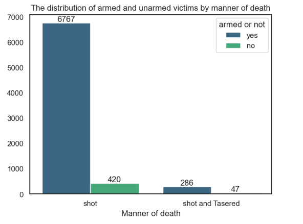
Comment:
The majority of victims died from gunshot wounds, while tasers were used in only 333 cases. Armed victims are shot 16 times more often than unarmed victims. Additionally, they are six times more likely to be killed by taser use.
Showing Mental Illness and Manner of Death
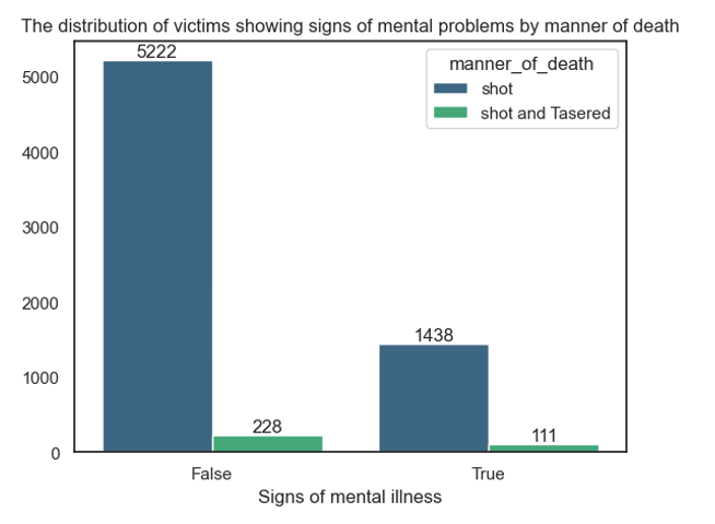
Comment:
The majority of victims in this dataset did not exhibit any signs of mental illness. However, among those who did show signs, tasers were used more frequently than gunshots in fatal encounters.
Armed and Manner of Death
Chi-squared Test
Null Hypothesis: Is there any association between manner of death and being armed?
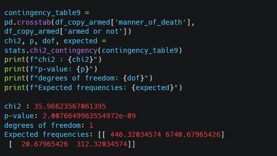
Comment:
The p-value of 2.01e-09 is much lower than the typical significance level (e.g., 0.05), allowing us to reject the null hypothesis. This means there is an association between being armed and manner of death.
Signs of Menal Illness and Manner of Death
Chi-squared Test
Null Hypothesis: Is there any association between manner of death and showing mental illness?
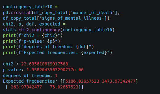
Comment:
With a p-value lower than 0.05,we ca reject the null hypothesis. This suggests that there is statistically significant association between signs of mental problems and manner of death in this dataset.
– What is the relationship between being armed or showing signs of mental illness and the manner of death in police shootings?
The chi-square tests show that there are significant associations between manner of death and signs of mental illness or being armed.
* Showing signs of mental problems increase the risk of being shot.
* Armed victims are shot 16 times more often than unarmed victims.
4.6 Are there geographic hotspots (by states) where police shootings occur more frequently? How does this correlate with other factors?
State
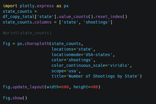
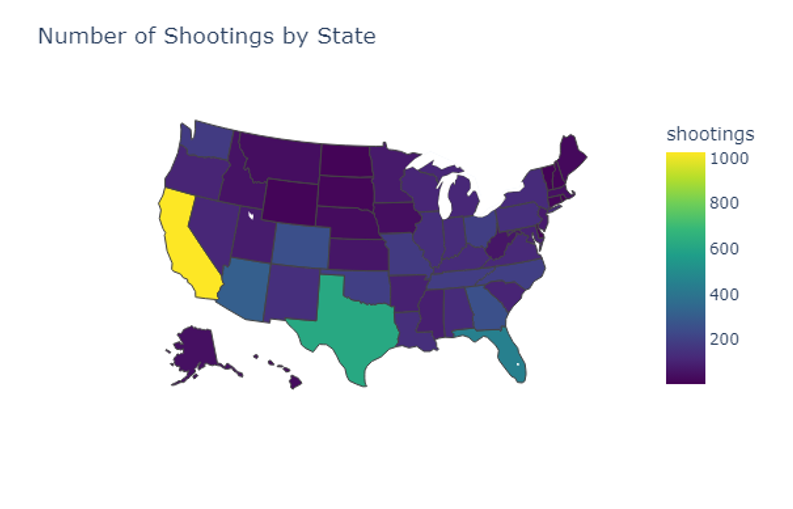
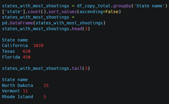
Comment:
The data reveals a significant disparity, with California having the highest number of shootings at a total of 1,028 cases, significantly outpacing other states. Texas, with 620 cases, ranks second in terms of shooting incidents. In contrast, states such as Rhode Island (5 cases), Vermont (11 cases), and North Dakota (15 cases) experience police shootings much less frequently. This chart illustrates the notable imbalance in shooting incidents among states, which may result from differences in population size.
State vs Age of Victims

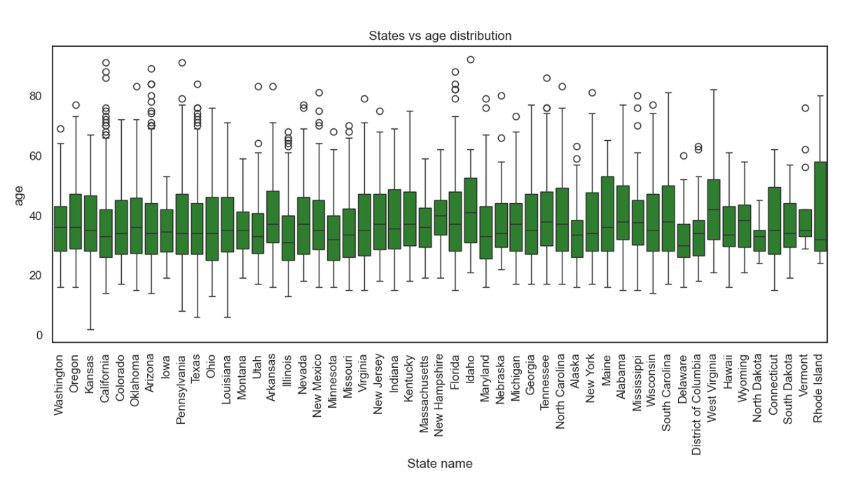
Comment:
Most victims’ ages fall between 20 and 60 years across the states, with the median age generally hovering around 30-40 years.
Some states, such as Louisiana and New Mexico, have wider interquartile ranges, indicating a broader spread of ages.
States like New York and Rhode Island show less variability, with most victims’ ages concentrated around the median.
While there are differences in the age spread and median values, no state shows an extreme departure from the overall trend.
State vs Fleeing Intention
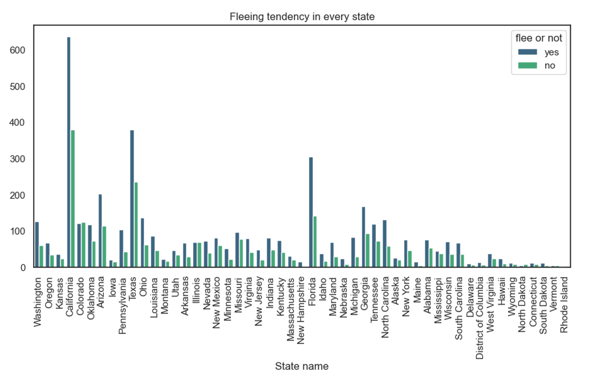
Comment:
· California and Texas stand out with the highest overall numbers of incidents, regardless of fleeing tendency. In California, a significantly larger number of individuals did not flee, while in Texas, there is a more balanced distribution between those who fled and those who did not.
· Washington, Florida, and Arizona also show notable numbers of individuals who fled compared to those who did not, with Washington having a particularly high number of fleeing incidents.
· States like New Hampshire, Nebraska, and Massachusetts show higher fleeing rates compared to non-fleeing incidents, while in most other states, the tendency not to flee appears more common.
· Smaller states like Rhode Island, South Dakota, and North Dakota have very few police shootings recorded, with a negligible difference between the number of fleeing and non-fleeing incidents.
This chart suggests significant variability across states in terms of fleeing tendencies during police shootings. States with higher populations, such as California and Texas, naturally have more incidents, but there is a noticeable variance in fleeing behavior between states. This could indicate differences in how law enforcement operates or how individuals react in various states during police encounters.
State vs Being Armed
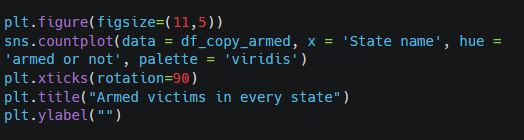
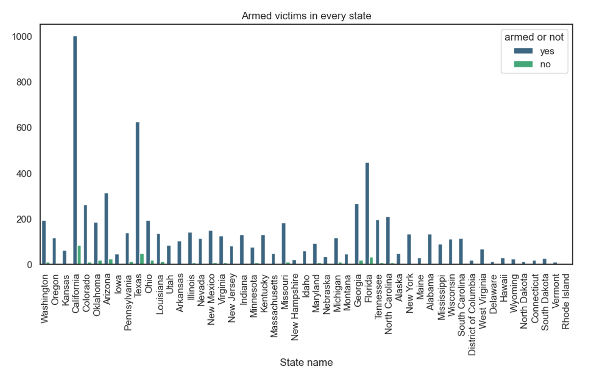
Comment:
· California has the highest number of armed victims, with nearly 1,000 armed individuals involved in police shootings. Very few unarmed victims are represented.
· Texas and Florida also have high numbers of armed victims compared to unarmed ones, with Florida showing a slightly larger share of unarmed victims than other high-incident states.
· Washington, Arizona, and Georgia show moderate numbers of armed victims, with some states like Oklahoma and Colorado having significant disparities between armed and unarmed victims, favoring more armed incidents.
· Several states such as Rhode Island, North Dakota, and South Dakota show very few incidents overall, both armed and unarmed.
· The general trend indicates that in almost every state, the majority of police shootings involve armed individuals, with relatively fewer incidents where the victim was unarmed.
State vs Being Armed
Chi-squared Test
Null Hypothesis: There is no association between state and being armed.
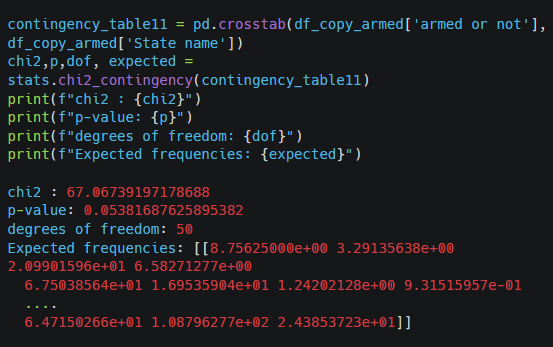
Comment:
The test results (p = 0.0538) suggest that there is no strong evidence of an association between being armed and the state in which the police shooting occurred, though the p-value is very close to 0.05.
State vs Age of Victims
Chi-squared Test
Null Hypothesis: There is no association between state and age of victims.
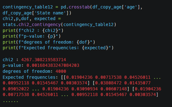
Comment:
A p-value this small strongly suggests that we should reject the null hypothesis. This means there is evidence to conclude that age of victims is associated with the state in which the police shooting occurred. While age and state are associated, this does not necessarily mean that state causes differences in age distribution. It might reflect other underlying factors (e.g., population demographics, regional trends).
State vs Fleeing Intention
Chi-squared Test
Null Hypothesis: There is no association between state and fleeing intention of victims.
Comment:
A p-value of 0.00018 strongly suggests that we should reject the null hypothesis. This means there is evidence to conclude that state is associated with the likelihood of flee in the data.
It might be valuable to explore which states specifically deviate from the expected fleeing patterns.
California has the highest number of shootings at a total of 1,028 cases, significantly outpacing other states. Texas, with 620 cases, ranks second in terms of shooting incidents. In contrast to them, states such as Rhode Island (5 cases), Vermont (11 cases) very rarely are a place of police shooting with death effect.
There are differences in the age spread and median values, but no state shows an extreme departure from the overall trend (around 30-40 years). The result of chi-square test concludes that age of victims is associated with the state in which the police shooting occurred.
The test showed also that there is no strong evidence of an association between being armed and the state.
Armed individuals are disproportionately involved in police shootings across the U.S., particularly in high-population states such as California, Texas, and Florida. States with lower populations show fewer incidents, and the number of unarmed victims remains consistently low across all states.
5. Results Analysis
Race, Gender, and Age: Black individuals and Native Americans are overrepresented in police shootings compared to their population sizes. Males dominate the victim pool across all racial groups, particularly White and Black individuals. Most victims are aged 20 to 50, with the Native group skewing younger and White victims showing a broader age range.
Armed Status and Mental Illness: Armed individuals are 16 times more likely to be shot, and males are more likely to be armed. There is a strong association between race and being armed—White victims had the highest number of armed cases, while Black individuals showed a higher proportion of unarmed victims. Mental illness is also linked to an increased likelihood of being shot.
Fleeing: Black individuals had the highest rate of fleeing attempts, while younger victims across all races were more likely to flee than older ones.
Geography: California has the most police shootings, followed by Texas. Smaller states like Rhode Island and Vermont rarely experience such incidents. Age distribution is fairly consistent across states, and while being armed is not strongly associated with location, larger states have higher numbers of both armed and unarmed shootings.
6. Conclusions
The analysis highlights significant racial, gender, and geographic disparities in fatal police shootings. Black and Native American individuals are disproportionately affected relative to their population sizes, and males overwhelmingly dominate the victim pool. Armed individuals and those showing signs of mental illness are at much higher risk of being fatally shot. Additionally, younger individuals are more likely to attempt fleeing, especially among Black victims.
Implications
These results suggest a need for more targeted intervention strategies, particularly addressing the racial and mental health disparities in police encounters. There is also a need for reviewing the use of force protocols, especially in cases involving armed individuals and those with mental health issues.
Future Research
Further studies could explore the factors behind the racial and gender disparities in greater detail, as well as the role of law enforcement practices in different states.
7. Additional Information
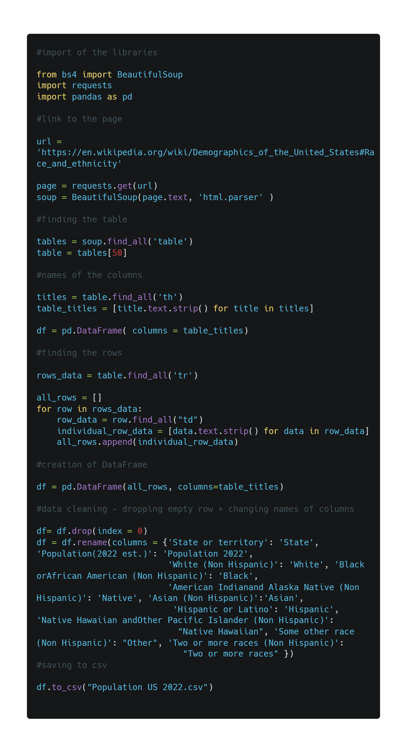
Population Data Scraping
To obtain the 2022 population figures for the United States, I conducted web scraping from Wikipedia (https://en.wikipedia.org/wiki/Demographics_of_the_United_States#Race). For this purpose, I developed a script utilizing the BeautifulSoup library:
Power Bi Dashboard
I created few measures in order to add some interesting facts and statistics to the dashboard. Examples:
- The flee % measure calculates the percentage of incidents in which individuals fled (flee) during police shooting events in the dataset from the table ‘shootings clean’.
flee % = DIVIDE(COUNT(‘shootings clean'[flee]), CALCULATE(COUNT(‘shootings clean'[flee]),
ALL(‘shootings clean’), ‘shootings clean'[flee] <> BLANK()))
- In order to calculate the percentage of victims that showed signs of mental illnesses, I divided the number of these individuals by the total number of cases.
With Signs = CALCULATE(COUNTROWS(‘shootings clean’), ‘shootings clean'[signs_of_mental_illness] = «true»)/’shootings clean'[Total]